Project Portfolio

BOLD fMRI Prediction

April 2025 - May 2025

Code available upon request.

Description:

This project explores how the human brain processes natural language by developing several predictive encoding models that map textual features of spoken stories to brain activity (fMRI Blood-Oxygen-Level-Dependent responses). Building on prior work by Huth et al., we evaluate different embedding strategies to improve prediction accuracy and gain insights into how linguistic context and hierarchical representations influence brain activity. The findings could enhance our understanding of language localization in the brain and have future applications in brain-computer interfaces and language disorder diagnostics.

We knew that traditional word embedding strategies would be effective, but unhelpful when accounting for contextual understanding. Thus, we developed 5 models to compare:

Traditional Embedding Methods:

One-Hot Encoding – To create the OHE embeddings, we mark each word that appears in the story as a 1 with respect to a word bank, and leave all words that don’t appear as 0. Similar to bag-of-words.
Word2Vec – These models are shallow, two-layer neural networks that are trained to reconstruct linguistic contexts of words. Word2vec takes as its input a large amount of text and produces a mapping of the set of words to a vector space, typically of several hundred dimensions, with each unique word in the group being assigned a vector in the space.
GloVe – constructs a word co-occurrence matrix where each element reflects how often a pair of words appears together within a given context window. It then optimizes the word vectors such that the dot product between any two word vectors approximates the pointwise mutual information (PMI) of the corresponding word pair.

Deep Learning Embedding Methods (contextual):

Initial BERT-style Masked Language Model – We leveraged PyTorch to build & train a BERT-style masked language model (MLM) encoder to generate contextual embeddings using the provided stories. These embeddings attempt to capture nuanced semantic and syntactic information based on the surrounding context. By aligning BERT embeddings with fMRI timepoints, we evaluated how well contextualized representations predict brain activity compared to traditional static embeddings.
Pretrained and Fine-tuned BERT-style Masked Language Model – Because MLMs require a massive amount of data and time to train, we fine-tuned a pre-trained BERT-style MLM on our specific story dataset to better capture the linguistic patterns. Fine-tuning allowed the embeddings to adapt to the nuances of the spoken narratives, potentially improving the alignment between textual features and fMRI responses. We compared prediction accuracy between the pretrained and fine-tuned models to assess the impact of domain adaptation on brain activity modeling.

Read more about our results in our project paper!

Arctic Cloud Classification Autoencoder

February 2025 - March 2025

link to project

Code available upon request.

Description:

This project addresses the challenges of accurately detecting cloud coverage in the Arctic, where snow, ice, and clouds have similar visual characteristics. Traditional satellite imagery struggles in polar regions due to uniform color and temperature, but the Multi-angle Imaging SpectroRadiometer (MISR) sensor improves detection by capturing data from nine different angles. In this project we leverage deep learning, feature engineering, and gradient boosting to create highly accurate (>98%) classifications of cloud and non-cloud pixels.

Autoencoder

We leveraged PyTorch to build a 6-layer autoencoder with convolutional layers. Because we wanted to maximize reconstriction accuracy, we didn’t reduce the original size of images (set stride to 1 for each layer). To do so without running out of GPU memory, we processed the images in 9x9 patches at train time.

Once fully trained, we downloaded the latent embeddings into CSV files, and eventually joined them with their associated pixels. Using the most “important” embeddings as features and engineered features, we then were able to utilize machine learning models for cloud prediction.

Feature Engineering

We decided to engineer a feature that combined the 3 “most important” features of the perimeter pixels of the current pixel. The idea behind this decision was that cloud pixels are close to one another these can help our final model better know about what’s close by. To find the most important features, we leveraged a decision tree to determine the feature importance of each angle’s features.

Gradient Boosted Model

After a lot of consideration and training, the final model we chose was a gradient boosting classifier with 63 leaves since it had the highest cross-validation F1-score (0.87). And after training this model with the entire training set, it had an F1-score of 0.944, an accuracy of 0.985, a precision of 0.914, and a recall of 0.977 with the test set.

Read more about our results in our project paper!

Adaptive Rejection Sampler

November 2024 - December 2024

Code available upon request.

Description:

Adaptive rejection sampling is a computationally efficient algorithm that allows sampling of log-concave probability density functions. Like the name suggests, ARS is relatively similar to rejection sampling except we can manipulate the log-concavity to create “squeeze” and “envelope” linear functions that limit both the number of samples we have to throw away and the number of evaluations of our probability density function. This can be particularly useful in cases where evaluation of the pdf is expensive and when sampling a truncated distribution.

Algorithm:

Initialize some abscissa \(T_k\), and calculate breakpoints \(z_k\), where \(z_0\) is the lower bound of the domain \(D\)¸

while number of samples desired not reached:

Calculate the envelope and squeeze functions at abscicca points, as well as a sample function \(s_k\), which is the exponentiated and normalized envelope.

Draw some \(w \sim \textnormal{Uniform}(0, 1)\) and \(X^{\star} \sim s_k\)

if \(w \leq \exp(l(X^{\star}) - u(X^{\star}))\) accept \(X^{\star}\) and return to begining of while loop.

otherwise, calculate the log pdf and derivative log pdf values of \(X^{\star}\), \(h(X^{\star})\), and \(h^\prime(X^{\star})\).

if \(w \leq \exp(h^\prime(X^{\star}) - u(X^{\star}))\) accept \(X^{\star}\)

add \(X^{\star}\) to the abscissa

Example:

How the algorithm works with an unnormalized normal density:

import numpy as np
import matplotlib.pyplot as plt
import seaborn as sns
import ars

def alpha_normal_pdf(x, mu, var):
    return np.exp((-1 / (2*np.sqrt(var)) ) * (x - mu) ** 2)
    
def plot_h_l_u(T, hvals, h, hprimes, z_ext):
    x_vals = np.linspace(z_ext[0], z_ext[-1], 500)
    # envelope
    u = ars.utils.get_u(T, hvals, hprimes, z_ext)
    # squeeze
    l = ars.utils.get_l(T, hvals)

    h_y = np.array([h(x) for x in x_vals])
    u_y = np.array([u(x) for x in x_vals])
    l_y = np.array([l(x) for x in x_vals])

    plt.figure(figsize=(10, 6))
    plt.plot(x_vals, h_y, label='log density', color='blue', linewidth=2)
    plt.plot(x_vals, u_y, label='envelope', color='red', linestyle='--')
    plt.plot(x_vals, l_y, label='squeeze', color='green', linestyle=':')
    plt.scatter(T, hvals, color='black', label='abscissa', zorder=5)
    plt.legend()
    plt.xlabel('x')
    plt.ylabel('Function values')
    plt.title('h(x), u(x), and l(x)')
    plt.grid(True)
    plt.show()

Here we will initialize the abscissa as -2 and 2. The z, and hprime calculations are all available in the source code upon request. Here is a visual representation of the squeeze and envelope functions that provides some intuition.

T = [-2, 2]
z_ext = [-2, 0, 2]
h = lambda x: np.log(alpha_normal_pdf(x, 0, 1))
hvals = [-2, -2]
hprimes = [2, -2]
plot_h_l_u(T, hvals, h, hprimes, z_ext)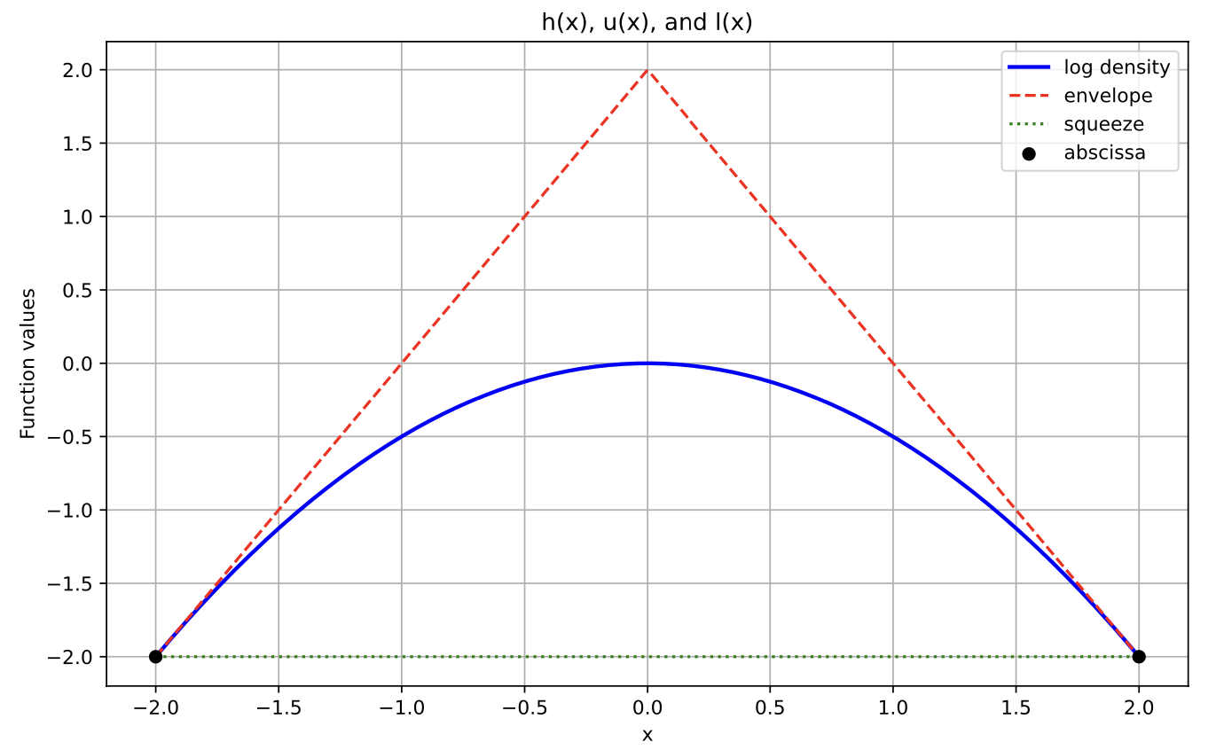

With another point in the abscissa (might occur if we rejected some \(X^\star=0\) during the initial squeeze test):

T = [-2, 0, 2]
h = lambda x: np.log(alpha_normal_pdf(x, 0, 1))
hvals = [-2, 0, -2]
hprimes = [2, 0, -2]
z_ext = ars.utils.get_z_ext(T, hvals, hprimes, 2, -2)
plot_h_l_u(T, hvals, h, hprimes, z_ext)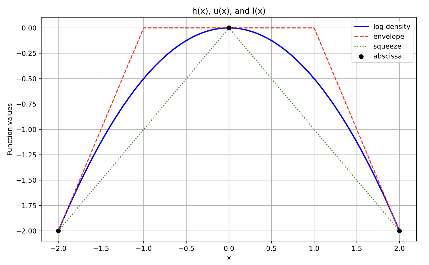

Now suppose we wanted to sample some truncated normal distribution between -2 and 0. We could simply use our ars method to create and plot 3000 samples:

from scipy.stats import truncnorm
std_normal_pdf = lambda x: alpha_normal_pdf(x, mu=0, var=1)
# Domain
D = (-2, 0)

sampler = ars.Ars(pdf=std_normal_pdf, D=D)
samples = sampler.ars(3000)

# Truncated Normal PDF from scipy for overlay
a, b = (D[0] - 0) / 1, (D[1] - 0) / 1  # Normalized bounds for standard normal
x_vals = np.linspace(D[0], D[1], 500)
truncated_pdf = truncnorm.pdf(x_vals, a, b, loc=0, scale=1)

plt.figure(figsize=(10, 6))
plt.hist(samples, bins=30, density=True, alpha=0.6, color='blue', label='ARS Samples')
plt.plot(x_vals, truncated_pdf, 'r-', lw=2, label="Truncated Normal PDF")

plt.title("Histogram of ARS Samples with Truncated Normal Overlay", fontsize=16)
plt.xlabel("x", fontsize=14)
plt.ylabel("Density", fontsize=14)
plt.legend()
plt.grid(True, linestyle='--', alpha=0.5)


plt.tight_layout()
plt.show()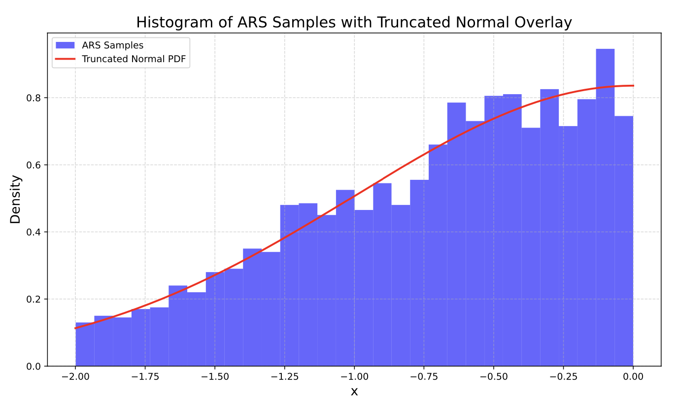

What I Learned

Enhanced teamwork and collaboration by effectively utilizing Git and GitHub for version control.
Developed a comprehensive Python package, incorporating well-structured modules, clear documentation, and robust functionality to address specific programming needs or streamline workflows.
Improved understanding of simulation, using Inverse Transform Sampling to sample from the normalized exponential envelope function.

Gradebook

January 2024 - June 2024

Code available upon request.

Description:

Gradebook is an open-source R package and Web Application that provides a consistent interface for instructors to quickly and more accurately calculate course grades.

The Problem: Many instructors (especially at Berkeley) opt to use Gradescope for students to upload their submissions to course assignments, as it provides an industry leading interface to instructors and readers for grading. However, Gradescope lacks functionality of implimenting a course policy. An example of a course policy (Data 88S):

At first, this might seem like a simple problem to solve with some sort of code file (perhaps using Pandas & NumPy in Python or R). But we have seen with courses such as Statistics 20 that these course policies can get extraordinarily convoluted and error prone.

The current best solution for instructors to calculate final grades based on their course policy is to either of the following:

Parallel program two seperate code books and compare the scores against one another until they agree.
- pros: very accurate
- cons: takes two programmers that fully understand the course policy & takes longer than single code book.
Create a single code book that can result in potential bugs that result in inaccurate scores.
- pros: faster than parallel programming
- cons: error prone and still not a fast solution.

The Solution:

Gradebook: An interface that abstracts the code into human understandable steps.

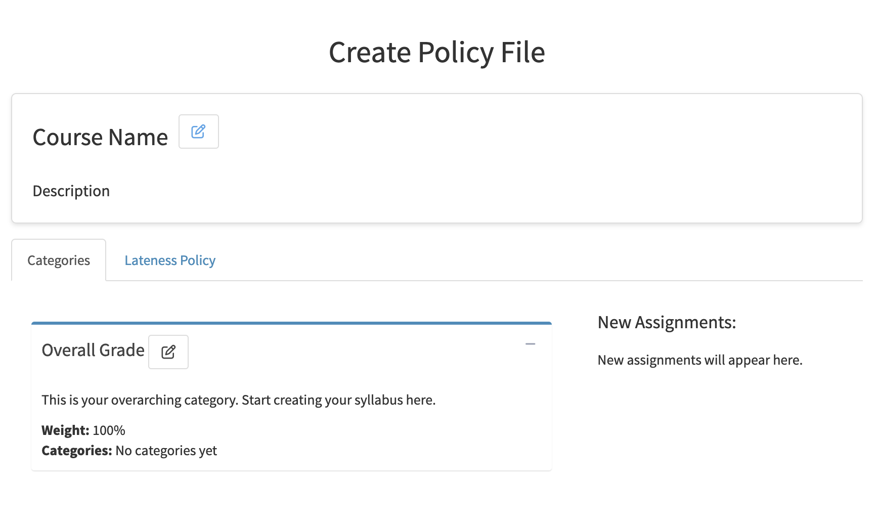
An instructor (or reader) provides the web app with their course policy using the intuitive policy tab. Then, they can upload their course’s Gradescope CSV to see data visualizations, statistics, a final grade table, and more.

What I Learned

During my time with the Gradebook team, I was responsible for designing and developing the “Dashboard” which displays graphics and statistics so the instructor can visually gauge their student’s project.

Applying Data Visualization skills using Plotly.
Git and GitHub (including branching, pull requests, working with github in a team setting).
The importance of Teamwork & Communication in Data Science.
Web development essentials (incl. HTML, CSS)

Email Spam Detection

November 2023, February 2024

Code available upon request.

Description: In my time as an undergraduate at Berkeley, I’ve had a few projects address the famous problem of email spam detection. In two seperate semesters, I created both a Logistic Regression and a Support Vector Machine model.

Logistic Regression

To find the best features for my model, I used exploritory data analysis techniques, including visualization with a heatmap of the feature correlations, bivariate data analysis with data visualization, and filling NA values in features with appropriate aggregations (mean, median, or 0 depending on skew of univariate distribution).

I also used feature engineering to get some of the most effective features for my regression. Some of the best features I found were the following:

Email is a “forwarded” or “reply” *.
Length of subject line in email.
Overall “wordiness” of email *.
Proportion of capital letters in subject line *.

* - Engineered feature.

Resulting ROC Curve:

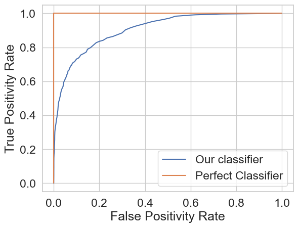
My final test accuracy using this model was \(\approx\) 87%.

Support Vector Machine (SVM)

Used k-fold cross validation to optimize C value in svm.SVC function found in the scikit-learn package in Python. Eventually landed on a test accuracy of 86% using the rbf kernel with a C value of 325.

What I Learned

Logistic Regression, including cross entropy loss, logit function, and interpretation.
Further developed knowledge of the scikit-learn tool basket.
Soft-margin Support Vector Machines (SVMs), who introduces flexibility by allowing some margin violations (compare to hard-margin who don’t).

Diabetes Classification

December 2023

https://github.com/calv2n/diabetes-risk-model

Description: In this project, I gathered data about diabetes patients from Kaggle and made accurate models for diagnosis given some common indicators. For my models, I wanted high accuracy and interpretability so we can see why the model chose what it chose. This is why I decided to use two seperate models: Logistic Regression and the Random Forest Classifier.

EDA: In the exploratory data analysis portion of building these models, I wanted to find the best way to visualize the best features for prediction. To do so, I created a heatmap of the absolute valued correlation between each feature and the diagnosis.

sns.heatmap(df.corr()['Diabetes'].abs().sort_values().to_frame(), annot=True);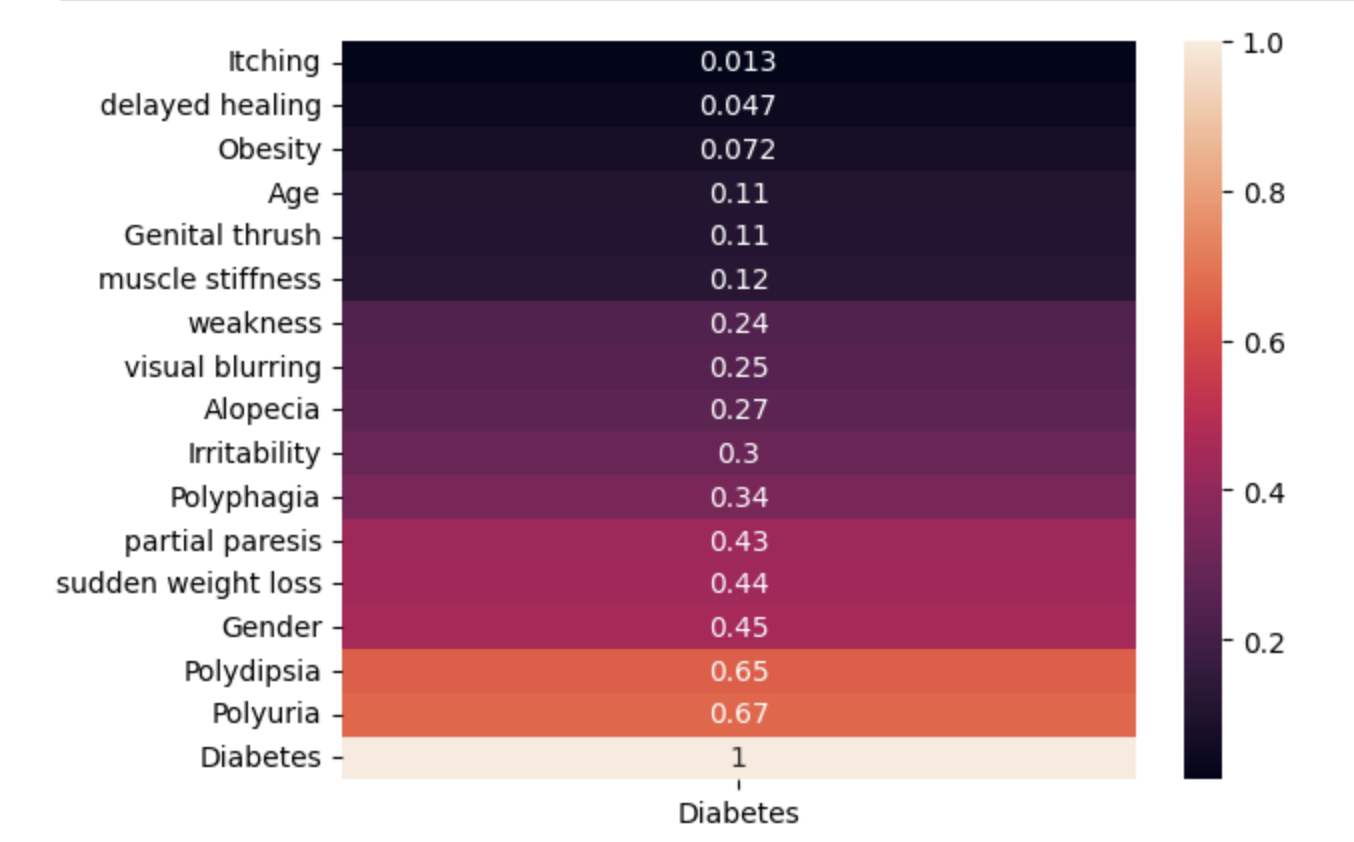

From here, I decided to use all of ‘Age’, ‘Gender’, ‘Polyuria’, ‘Polydipsia’, ‘sudden weight loss’, ‘weakness’, ‘Polyphagia’, ‘Genital thrush’, ‘visual blurring’, ‘Irritability’, ‘partial paresis’, ‘muscle stiffness’, ‘Alopecia’, and ‘Obesity’ to make my predictions.

Logistic Regression

from sklearn.linear_model import LogisticRegression

model = LogisticRegression(max_iter=500)
model.fit(X_train, y_train)
train_prediction = model.predict(X_train)
val_prediction = model.predict(X_val)

train_accuracy = np.mean(train_prediction == y_train)
val_accuracy = np.mean(val_prediction == y_val)

print(f'Model training accuracy: {train_accuracy}')
print(f'Model validation accuracy: {val_accuracy}')

Model training accuracy: 0.9302884615384616 
Model validation accuracy: 0.9038461538461539

Highlights:

>90% validation accuracy using a human interpretable model.
Modified threshold to supremum such that the model’s recall was 100% (important to minimize false negatives in many healthcare settings) while keeping validation accuracy > 85% (see chunk 57).

Random Forest Classifier

from sklearn.ensemble import RandomForestClassifier

m2 = RandomForestClassifier(random_state=42)
m2.fit(X_train, y_train)

m2_val_prediction = m2.predict(X_val)

print(f'Model Validation Accuracy: {(tp + tn) / (tp + tn + fp + fn)}')
print(f'Model Precision: {tp / (tp + fp)}\nModel Recall: {tp / (tp + fn)}')

Model Validation Accuracy: 0.9807692307692307
Model Recall: 1.0
Model Training Accuracy: 1.0

Highlights:

>=99% validation accuracy, though not human interpretable.
Keeps highest possible validation accuracy while keeping recall at 100%.

What I Learned

How to manipulate prediction threshold in code to maximize recall.
The importance of maximizing recall in a diagnosis setting. It’s way more dangerous (and potentially life threatening) to wrongly tell someone that they don’t have a disease when they do in reality.
The “tradeoff” of interpretability and accuracy in machine learning.
I used this project as an oppertunity to explore the implementation of random forest models. I learned how they worked in theory how they worked in Data 102 and from there thought they were very interesting.
Why (in practice) symptoms like constant urination and obesity are considered common symptoms of diabetes.

Gitlet

July 2023

Code available upon request.

Successfully Implemented the following commands from the Git Version Control System:

init: Creates a new Gitlet version-control system in the current directory.
add: Adds a copy of the file as it currently exists to the staging area.
commit: Saves a snapshot of tracked files in the current commit and staging area so they can be restored at a later time, creating a new commit.
restore: Restore is used to revert files back to their previous versions. Depending on the arguments, there’s 2 different usages of restore:
1. java gitlet.Main restore -- [file name]
2. java gitlet.Main restore [commit id] -- [file name]
log: Starting at the current head commit, display information about each commit backwards along the commit tree until the initial commit, following the first parent commit links, ignoring any second parents found in merge commits.

===
commit a0da1ea5a15ab613bf9961fd86f010cf74c7ee48
Date: Thu Nov 9 20:00:05 2017 -0800
A commit message.

===
commit 3e8bf1d794ca2e9ef8a4007275acf3751c7170ff
Date: Thu Nov 9 17:01:33 2017 -0800
Another commit message.

===
commit e881c9575d180a215d1a636545b8fd9abfb1d2bb
Date: Wed Dec 31 16:00:00 1969 -0800
initial commit

global-log: Like log, except displays information about all commits ever made.
rm: Unstage the file if it is currently staged for addition. If the file is tracked in the current commit, stage it for removal and remove the file from the working directory if the user has not already done so.
find: Prints out the ids of all commits that have the given commit message, one per line. If there are multiple such commits, it prints the ids out on separate lines.
status: Displays what branches currently exist, and marks the current branch with a *. Also displays what files have been staged for addition or removal.
branch: Creates a new branch with the given name, and points it at the current head commit.
switch: Switches to the branch with the given name. Takes all files in the commit at the head of the given branch, and puts them in the working directory, overwriting the versions of the files that are already there if they exist. Also, at the end of this command, the given branch will now be considered the current branch (HEAD). Any files that are tracked in the current branch but are not present in the checked-out branch are deleted. The staging area is cleared, unless the checked-out branch is the current branch.
rm-branch: Deletes the branch with the given name. This only means to delete the pointer associated with the branch; it does not mean to delete all commits that were created under the branch, or anything like that.
reset: Restores all the files tracked by the given commit. Removes tracked files that are not present in that commit. Also moves the current branch’s head to that commit node.

What I Learned

This was my first large project when I came to Berkeley as an undergraduate.

Java for large scale projects
Designing and implimenting data structures to maximize efficiency.
Fundamentals of Git as a software from the ground up.